Optimal entanglement witnesses for continuous-variable systems

In the experimental study of continuous-variable entanglement is it often tremendously helpful to employ criteria for entanglement based on second moments, so on "variances", of canonical coordinates or quadratures. The typically used criteria correspond to hyperplanes in the set of second moments. If one aims at detecting instances of multi-particle entanglement in many modes, or entanglement in locally squeezed states, it can be very involved to find appropriate tests. 

Yet, recently it has turned out that the set of all such hyperplanes can be completely characterized (unlike the entanglement witnesses as observables in the sense of hyperplanes to the set of separable states). Also, to find an optimal test based on second moments most robust against noise for a given "guessed" state can be extracted from the solution of certain semi-definite programs. Further, curved product criteria can be constructed from the solutions. Here, we present a software package, consisting of the functions FULLYWIT and MULTIWIT, that finds such optimal test, both for bi-partite and multi-partite settings. 

The associated theoretical work, as well as documentation of the software, can be found under this link.

Percolation on a diamond lattice

This page outlines some features of percolation on a diamond lattice - its main purpose is to provide extra information regarding the constructions which are mentioned somewhat briefly in the paper: Percolation, renormalization, and quantum computing with non-deterministic gates, by Konrad Kieling, Terry Rudolph, and Jens Eisert. This entry is a mirror of the entry of this site.

Disclaimer: The matlab code here is not particularly efficient, and it is not the code which was used to perform the simulations mentioned in the paper. This code is given so that an interested reader can easily play around with (and visualize) percolation on the diamond lattice, and obtain some understanding some of the graph theoretic methods necessary to deal with the intrinsic randomness of the resultant cluster states.

Introduction to the basic ideas

This project is about using ideas from percolation theory to deal with issues that arise in practical implementations of quantum information. More precisely, it covers statements on the scaling behaviour that arises when cluster states are generated with means of probabilistic gates, small initial resources, the positions of which during the whole procedure are fixed. So, we are using a static setup without any re-routing (aka active switching or coherent feed-forward). Interestingly, it is shown that even with these quite strong restrictions, one can come as close as desired to the optimal scaling of O(L²) resources for a cluster state of size LxL (that is, the scaling which would be attained were deterministic gates actually available). For more information on the proof of this statement or the whole problem as such, see quant-ph/0611140.

This page itself is centered around classical post-processing once the probabilistic entangling gates have been employed. We focus on the algorithms needed to extract graph states suitable for quantum computation from the percolated lattice, rather than arguments on the percolation, its scaling, or physical implementations.

In the race for small initial pieces we use the diamond lattice a basic star structure which can be used to build up this lattice. For computational simplicity, it is possible to embed the diamond lattice into a cubic lattice, thus allowing for easy indexing and addressing of sites (see the two figures below for diamond and its embedding into cubic).

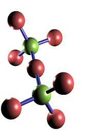
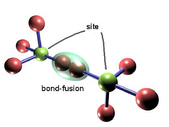
The green "center" qubits constitute the sites of the lattice to build, the red ones are merely there to be used in the probabilistic bond-fusion, giving rise to the bond percolation process discussed in the paper. Depending on the physical implementation, they might be completely measured out, or one of a pair might survive.

Setting up the lattice

The diamond lattice (it really is the lattice of carbon atoms in diamond!) consists of vertices arranged in 3-dimensional space; each vertex has 4 bonds emanating from it. In the cubic embedding we take the vertices ("sites") to be at coordinates (i,j,k) where the values of i,j,k are integers ranging from 1 to integers Lx,Ly,Lz respectively. If a vertex is even (i+j+k is even) then the direction vectors from that site are

{(1,0,0),(-1,0,0),(0,1,0),(0,0,1)},

while if the site is odd then the direction vectors are

{(1,0,0),(-1,0,0),(0,-1,0),(0,0,-1)}.

One way we will represent the lattice is as a matrix of the edges (or "bonds"). Each row of the matrix corresponds to an edge - the first three columns refer to the coordinates of the first vertex of the bond, the second three columns are the coordinates of the second vertex. To avoid redundancies we can use the coordinate vectors only from the even sites. It is easy to build up a matrix encoding all the bonds as follows:

Lx=10;Ly=10;Lz=3;
allbonds=[];
for ii=1:Lx;for jj=1:Ly;for kk=1:Lz;
if floor(ii+jj+kk)/2==(ii+jj+kk)/2 %ie if site is even
allbonds=[allbonds;ii jj kk ii+1 jj kk;ii jj kk ii-1 jj kk;ii jj kk ii jj+1 kk;ii jj kk ii jj kk+1];
end;
end;end;end;

However matlab is bad with loops, so some more efficient code is the following:

Lx=10;Ly=10;Lz=3;
X=[repmat(1:Lx,Ly*Lz,1)];Y=[repmat(1:Ly,Lz,Lx)];Z=[repmat(1:Lz,1,Lx*Ly)];
INDX=[X(:),Y(:),Z(:)];
SINDX=sum(INDX')/2;
IE=find(floor(SINDX)-SINDX==0);
EVEN=INDX(IE,:);

allbondsijk=[EVEN, EVEN(:,1)+1, EVEN(:,2:3); EVEN,EVEN(:,1), EVEN(:,2)+1, EVEN(:,3); EVEN,EVEN(:,1:2), EVEN(:,3)+1; EVEN, EVEN(:,1)-1, EVEN(:,2:3)];

allbondsijk(find(or(allbondsijk(:,4)>Lx,allbondsijk(:,4)<1)),:)=[];
allbondsijk(find(or(allbondsijk(:,5)>Ly,allbondsijk(:,5)<1)),:)=[];
allbondsijk(find(or(allbondsijk(:,6)>Lz,allbondsijk(:,6)<1)),:)=[];

The last three lines are to remove sites with coordinates that are less than 1 or greater than Lx,Ly,Lz.
Either way, the list of edges is then in the matrix allbondsijk, the first few rows of which look like this:

allbondsijk(1:13,:) =

1 1 2 2 1 2
1 2 1 2 2 1
1 2 3 2 2 3
1 3 2 2 3 2
1 4 1 2 4 1
1 4 3 2 4 3
1 5 2 2 5 2
1 6 1 2 6 1
1 6 3 2 6 3
1 7 2 2 7 2
1 8 1 2 8 1
1 8 3 2 8 3
1 9 2 2 9 2
.
.

The first row means the site at x=1,y=1,z=2 is joined to the one at x=2,y=1,z=2. The "ijk" in the variable name refers to the fact that the labelling of the sites is in terms of their spatial coordinates. Later on we will need to label the sites through a unique integer ranging from 1 to N - in that case we would call the matrix allbondsN for example.

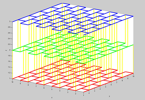
Below is a plot of the bonds on the diamond lattice. Here we have only produced 3 layers of the lattice in the Z-direction, so as to make visualizing it a bit easier. In the figure below different colors have been chosen for each Z-layer. As such it is easy to see that in this form the lattice consists of sheets of "brickwork" (which is the honeycomb lattice) with vertical connections between alternating sites.

Percolating the lattice

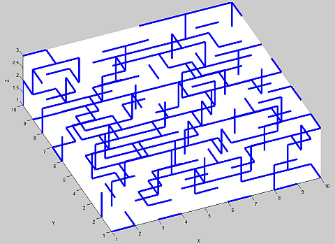
We now want to remove each bond from our complete diamond lattice with an independent probability p, which I will take to be 1/2. This mimics the process using photons and fusion (described above) in which a bond in the lattice becomes connected if a Type-I fusion between the two qubits lying along the bond succeeds. In matlab this is easily achieved, and the new matrix of the edges which survive is stored as connectedbonds:

R=rand(length(allbondsijk),1);
connectedbondsijk=allbondsijk(find(R<0.5),:);

Here is a plot of the bonds which remain for a typical example:

Finding the largest cluster in the lattice

Clearly some of the bonds in the above picture are "floating around" on their own, and will not be useful to us. We need to identify the clusters of connected bonds. In particular, since we are above the percolation threshold, we need to identify the (unique) "spanning cluster" - the set of bonds which, as we make Lx, Ly and Lz larger, are certain to exist and are guaranteed to provide a path from one side of the lattice to the other.

Fortunately there is an extremely efficient method for identifying all the clusters in a lattice. It is often known as the Hoshen-Kopelman algorithm (Phys. Rev. B, 14, 3438 (1976)) - it is basically what computer scientists call a depth first search. This method has the following nice features: It does not require knowing what is going on with the rest of the cluster in order to decide which cluster label to give any site. This means that it is particularly well suited to a situation where we grow a percolated graph state dynamically and compute with it as we go - something which would alleviate requirements on quantum memory, (but which we will not explore here!).

Although it is not too difficult to code up these algorithms, there is already a graph theory package for matlab - matlab_bgl - which is basically a set of matlab wrappers for the Boost Graph Library.

The problem with using this package - or pretty much any graph theory package - is that we need to input the graphs as a (sparse) adjacency matrix. For this we need to give each of the sites (which so far we have labelled with (i,j,k) coordinates) a unique vertex label ranging from 1 to some number N, which could be as large as Lx*Ly*Lz. Because this is a useful thing to be able to do, it makes sense to define a function:

function [bondsmatrixN,A,Q]=ijk2N(bondsmatrixijk)

%This function converts a bonds matrix in ijk form to one in which each site has a unique integer label. It also outputs an adjacency matrix A, and a matrix Q such that Q(n)=[i j k], where n is the integer label of site (x=i,y=j,z=k)

%The following line of code finds the unique (i,j,k) sites in the matrix E of ijk edges - the
%unique index for each site is simply which row it appears in the matrix Q:

Q=unique([bondsmatrixijk(:,1:3);bondsmatrixijk(:,4:6)],'rows');
N=size(Q,1); %number of sites

%We now go and find the corresponding row of Q for each site in the matrix
%"connectedbonds". This allows us to construct a new matrix of the edges -
%called "bondsmatrixN" - which uses a single integer for each of the site labels:

[irrelevant,edge1]=ismember(bondsmatrixijk(:,1:3),Q,'rows');
[irrelevant,edge2]=ismember(bondsmatrixijk(:,4:6),Q,'rows');
bondsmatrixN=[edge1,edge2];

% Finally we turn the edgelist into a (sparse) adjacency matrix:
A=spalloc(N,N,2*length(bondsmatrixN));
for ii=1:size(bondsmatrixN,1)
A(bondsmatrixN(ii,1),bondsmatrixN(ii,2))=1;
A(bondsmatrixN(ii,2),bondsmatrixN(ii,1))=1;
end

return

This function returns a 2 by |E| matrix of edges, an adjacency matrix A, and the indexing matrix Q which can sometimes be useful. In our main program we want to call this on our matrix connectedbondsijk:

[connectedbondsN,A,Q]=ijk2N(connectedbondsijk);

The N is there to denote that this is the matrix of connected bonds in the format where each site has an integer label from 1 to N, instead of an (i,j,k) label. The first few rows of connectedbondsN may look (depending on the results of the bond percolation of course) something like this:

connectedbondsN(1:10,:)=

7 91
8 92
13 98
15 100
18 103
21 107
28 113
30 115
36 121
38 123

We are now ready to call the components routine of the matlab_bgl library - this routine requires a sparse adjacency matrix input. The routine outputs a vector sitelabel which is the label for each site in the graph with adjacency matrix A. Two sites have the same label iff they are part of the same connected piece of the graph. The routine also outputs the size of the connected component associated with that label. So to find the largest cluster we find the label which has the most sites, and then find all vertices with that label:

[sitelabel,sizes]=components(A);
[largestclustersize,largestclusterlabel]=max(sizes);
largeclustervertices=find(sitelabel==largestclusterlabel);

We then go through and extract out a new matrix of edges, which contains only edges where the sites are part of the largest cluster:

IA1=find(ismember(connectedbondsN(:,1),largeclustervertices)>0);
IA2=find(ismember(connectedbondsN(:,2),largeclustervertices)>0);
largestclusterijk=connectedbondsijk(intersect(IA1,IA2),:); %note this is ijk form

Here is a plot of an example where Lx=Ly=Lz=10. The largest connected cluster has been colored black - the next two largest ones are colored red and green.

Finding paths through the largest cluster

We are now at the point where we want to find paths through the spanning cluster. In the paper we described a blocking procedure, wherein you take the large spanning cluster and chop it into blocks of size B in the x,y directions (so the number of blocks is Lx/B etc), but keep the whole block in the z direction. For example, the first block consists of those sites with coordinates (1≤i≤B,1≤j≤B, 1≤k≤Lz) for the chosen value of B. In fact there are many ways to proceed from here, some apparently more efficient than what we describe in the following, although this seems the most intuitive approach.

It turns out there is a whole industry of computer scientists producing algorithms that find paths between vertices in graphs. These algorithms go by names such as djisktra, A* and many others, thoughfor our purposes a simple simple breadth first search would suffice. In the case (such as we have) that the graph is given on some natural lattice geometry, then using various so-called "hueristics" can greatly speed up things. We will simply use the shortest_paths routine of the matlab_bgl package.

We will illustrate the procedure by taking the whole set of vertices in our spanning cluster as a single block. That is, our block is Lx by Ly by Lz in size.

First we convert the ijk form of the largest cluster to an adjacency matrix form:

[largestclusterN,A2,Q2]=ijk2N(largestclusterijk);

We then identify the midpoint of the block, and the midpoint of the face of the block defined by y=1:

midblock=[Lx/2,Ly/2,Lz/2];
midface1=[Lx/2,1,Lz/2];

We want the coordinates of the site which is part of the largest cluster and closest in Euclidean distance to midblock. The following piece of ugly code does it:

[mindistancemiddle,middlevertexN]=...
min(sum((abs(Q2-repmat(midblock,size(Q2,1),1)).^2)')');

middlevertexijk=Q2(middlevertexN,:)

We also want the coordinates of the site which is part of the largest cluster, and closest in Euclidean distance to midface1. We need to be careful however. We only want to consider sites that actually lie in the plane of that face - otherwise when we want to join adjacent blocks through their common face we will have a problem. So first we filter down to all the sites in that face, and then we find the one which is closest to the middle:

face1sites=Q2(find(Q2(:,2)==1),:);

[mindistanceface1,minindexface1]=...
min(sum((abs(face1sites-repmat(midface1,size(face1sites,1),1)).^2)')');

face1vertexijk=face1sites(minindexface1,:)

[irrelevant,face1vertexN]=ismember(face1vertexijk,Q2,'rows');

We have also output the index face1vertexN of this site in the "N-form", since this is what will be required to find the appropriate output from the shortest paths routine. We now call shortest_paths which actually finds all shortest paths from the specified originating vertex - in our case the middle site of the block - to every other vertex in the block:

[d1,parent]=shortest_paths(A2,middlevertexN);

Unfortunately the output to this routines is not a path explicitly, but rather what is known as a "predecessor" or "parent" vector. The n'th elelemnt of this vector tells you what is the previous site to go to, when following the shortest path back to the specified originating site - in our case middlevertexN. To convert this back to a path it is convenient to definte a function which turns predecessor vectors into paths:

function path=parent2path(parent,endvertex);
%converts a predecessor vector into a list of the sites traversed in the path
n=1;
v=endvertex;
while v~=0
path(n)=v;
v=parent(v);
n=n+1;
end

Our path from the middle of the block to the first face is then easily extracted:

path1=parent2path(parent,face1vertexN);
path1ijk=Q2(path1,:);

Repeating this for the other three faces, we find appropriate paths through the lattice. The output to path1ijk looks something like this:

path1ijk(1:13,:)=

4 1 5
4 2 5
5 2 5
5 3 5
5 3 4
4 3 4
4 3 3
4 4 3
4 4 2
4 5 2
3 5 2
3 5 3
3 4 3

A typical set of 4 paths looks like:

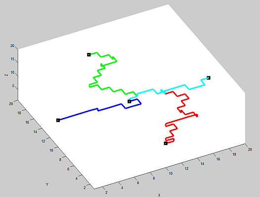
Clearly this whole procedure is easily iterated with the adjacent blocks, and large lattices can be built up efficiently.

Synopsis of the code, and some final useful functions:

Here are some matlab m files. The file "percolation_main.m" contains the code above. In addition it contains the code to produce the remaining three paths in the block, and at the end it contains some code to plot the various bond structures/paths etc. For plotting these bonds the function "bondsplot3d.m" given below is required. Also below are the two functions mentioned in the text above.

Download the zip file for all the Matlab code here.

Subtleties of the procedure and final remarks

We now have all the basic elements in place. We have a way of turning our percolated lattice into a simpler graph state: we simply measure out in the Z-basis all qubits which are not part of our identified paths. Although the resultant graph state has nontrivial topology (though without loops), we still need to argue that it is universal for quantum computing. The subtle part is that we do not (generally) get a 4-way junction from our chosen middle qubit. As the picture above shows, we will generally get 3-way T-junctions.

Although there might be ways to unite two T-junction into a cross by means of local measurements, we will go a conceptually more simple route. Instead of going directly for the crosses, we only generate a single T-junction per block. They are connected to the left and to the right faces and alternatingly to the top or to the bottom. The threads between these junctions can be shortened by employing double X-measurements and a Y-measurement, depending on the parity of the number of qubits between these junctions. In fact, the lattice that is generated with such a procedure is the hexagonal lattice, which in turn can be converted to a square lattice by using only local measurements.

Optimal strategies for fusing optical cluster states

The data available through this web page supplements the paper quant-ph/0601190.

We systematically investigate how to optimally build up cluster states for quantum computing with linear optical means using fusion gates, entirely from the perspective o f classical control. We develop a notion of classical strategies and consider the globally optimal one to prepare linear cluster states w ith probabilistic gates. We find that this optimal strategy - which is also the most robust with respect to decoherence processes - gives rise to an advantage of already more than an order of magnitude in the number of maximally entangled pairs when building chains with an expected length of L=40, compared to other legitimate strategies. For two-dimensional cluster states, we present a first scheme achieving the optimal quadratic asymptotic scaling in resource consumption. This analysis shows that the choice of appropriate classical control leads to a very significant reduction in resource consumption.

The files contain lines of the following format:

C, Q(C), Q(C) - \tilde Q(C), optimal action.

Here, C denotes a configuration, Q(C) the expected length of the final cluster state that results from acting on C by an optimal strategy, \tilde Q(C) is the expected final length that MODESTY would obtain and 'optimal action' lists the chains which an optimal strategy would fuse when confronted with C.

F or convenience the data has been grouped into files called 'tableXX.dat', where XX stands for N(C), the total number of edges in the respective configurations.

Please download the zip'ed data (15 MB).